How Risky is McDonald's Stock?

In finance, Value at Risk (VaR) is a crucial metric for assessing the risk of an investment portfolio. VaR provides an estimate of rare but potential loss an investment may face over a specific time horizon and confidence level. To calculate VaR, it’s necessary to have an understanding of the underlying distribution of investment returns.

To accurately determine this distribution, various models from time series analysis can be used. The GARCH model, in particular, is known for its effectiveness in analyzing financial data. One of the main reasons to choose GARCH over other models, such as empirical distribution (actually this is even model-free), random walk, or ARIMA, is that it can capture the volatility dynamics of the stock return, which is essential for accurate VaR calculation of financial asset return.

All models in time series analysis aim to explain future values of a time series using its past values, or lags. ACF and PACF are graphical tools used in time series analysis to identify the autocorrelation and partial autocorrelation at various lags of a time series, respectively. They are commonly used to determine the appropriate orders of the GARCH model by examining the decay of the autocorrelation and partial autocorrelation functions.

In this posting, I present the complete process for calculating daily VaR of McDonal’s stock including all the points mentioned above.

Prices, simple returns and log returns

Whose distribution exactly do we want to figure out for VaR calculation? Long story short, we identify the distribution of log returns of McDonald’s stock due to the desirable characteristics of log returns for statistical analysis purpose.

The terms “prices”, “simple returns” and “log returns” refer to different ways of measuring the performance of an investment over time. Price is the most common form of financial asset data we can encounter and the other two are transformed version of this. Let $P_{t}$, $R_{t}$ and $r_{t}$ respectively denote the price, one-period simple return and one-period log return of McDonald’s stock at time $t$. Then $R_{t}$ and $r_{t}$ are defined as

$R_{t}=\dfrac{P_{t}-P_{t-1}}{P_{t-1}}\tag{1}$

$r_{t}=log \left(\dfrac{P_{t}}{P_{t-1}}\right)=log(1+R_{t})\tag{2}$

The log return is frequently referred to as the continuously compounded return on account of the following mathematical principle.

Both $R_{t}$ and $r_t$ are measure of the relative movements of price, which is a useful property for comparison of performance between assets. Another technical reason we might be more interested in simple return and log return than raw price is that they could be used as a remedy for non-stationarity of price time-series (differencing).

Figure 1. Closing prices (top), simple returns (middle) and log returns (bottom) of McDonald's stock for past five years.

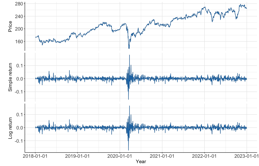
See A1 for the code to generate this figure.

As seen on the chart of McDonald’s stock price, it is impossible to conduct a statistical analysis with this due to the non-stationarity.

The substantial similarity simple return and log return charts exhibit is linked with the fact that the simple return metric is an approximation for log return by a first-order Taylor expansion. The first order Taylor Expansion of $log(x)$ around $x=1$ is as follows.

So, when $\dfrac{P_{t}}{P_{t-1}}\simeq 1$

When $R_{t}$ is small enough, the difference between simple return and log return is negligible. Log return, however, is often chosen over simple return at least for two practical reasons.

First, log returns are additive, which makes it simpler to calculate the total return of an investment over time. Let $r_{k,\ t}$ denote log return over $k$ period at time $t$, then it is defined as

Second, simple returns are inherently asymmetric due to the limited liability issue (simple returns are bounded by $-100\%$) and positive skewness, and logarithmic transformation remedies this problem by mapping the range of $(-1, 0)$ to the range of $(-\infty, 0)$ and limiting big positive values.

To summarize, log returns are often preferred in the statistical analysis of financial assets due to their suitability for comparison, symmetric nature, and ease of calculation for different time horizons. So, I will figure out the distribution of the log returns of McDonald’s stock for calculating Value at Risk (VaR).

Value at Risk (VaR)

Value at Risk (VaR) is the most broadly used risk metric in finance and is defined as follows.

$P(r_{k,\ t} \leq VaR_{k;\ 1-\alpha})=\alpha \tag{7}$

In plain English, equation $7$ states that the probability of an asset’s return over a given $k$ period, $r_{k,\ t}$ being less than or equal to the value of the VaR for that $k$ period at a confidence level of $1-\alpha$ is equal to $\alpha$. In other words, the VaR represents the maximum expected loss over a $k$ period with a confidence level of $1-\alpha$, or we have $\alpha$ probability of the expected loss going beyond the VaR. The most common values for $\alpha$ are $1\%$ and $5\%$, which are also universal values for significance level in hypothesis testing.

Figure 2.The empirical one period (daily) VaR of log returns of McDonald's stock with confidence level of $95\%$ is $-3.05\%$. In mathematical notation, $P(r_{t} \leq VaR_{95\%})=5\%$

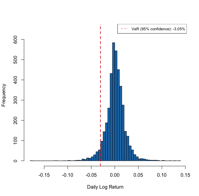
See A2 for the code to generate this figure.

What we are trying to figure out with VaR is also called “tail risk” and why it goes by the name is intuitively visualized on Figure $2$. The term “tail risk” is used to describe the potential for losses or extreme events that fall outside the normal range of outcomes and occur in the tails of a probability distribution.

The histogram drawn on Figure $2$ is like an empirical distribution, which is a probability distribution based on historical data rather than a theoretical model, which is why it is also called “model-free” distribution. The main assumption behind the choice to use empirical distribution for VaR calculation is that the probability distribution of returns in the past is a good representation of the probability distribution of returns in the future. This is not always valid, especially when the market is showing high volatility. Accurately characterizing the distribution of the data is crucial for VaR calculation, as the choice of distribution significantly impacts the accuracy of the calculated VaR. The issue poses the question, “What is the appropriate model that can accurately reflect the underlying distribution of the data?”

GARCH model with $t$-distribution

GARCH stands for Generalized AutoRegressive Conditional Heteroskedasticity, in which the conditional variance of the data is modeled against both autoregressive (AR) process and moving average (MA) process (Equation $9$, respectively blue and red). Let $X_{t}$ denote the time-series (in our case, log returns of McDonald’s stock), then we can assume the following GRACH $(p, q)$ structure.

$X_{t}=\mu+E_{t}=\mu+\sigma_{t}W_{t} \tag{8}$

$\sigma_{t}^{2} = \alpha_0 + \color{#5268DE}{\sum_{i=1}^{p}{\alpha_i E_{t-i}^{2}}} + \color{#DE5252}{\sum_{i=1}^{q}{\beta_i \sigma_{t-i}^2}} \tag{9}$

$W_{t} \sim t_{v}\left(0, \dfrac{v}{v-2}\right) \tag{10}$

$\mu$ is the constant conditional expectation and $E_{t}$ is an error term, which is a multiplication of the conditional variance, $\sigma_{t}^{2}$ and a White Noise innovation, $W_{t}$. The conditional variance, $\sigma_{t}^{2}$, has a GRACH $(p, q)$ structure in Equation $9$. $W_{t}$ is a random $iid$ variable from a standardized Student’s $t$-distribution with $v$ degrees of freedom, $t_{v}\left(0, \dfrac{v}{v-2}\right)$ or simply $t_{v}$.

We often use $t$-distribution as one of these so-called “heavy-tailed” distributions to incorporate the heavy-tailed property of the financial returns instead of the commonly used standard Gaussian distribution. Since Gaussian PDF decays rapidly with $e^{-x^{2}}$, $99\%$ observations appear within the range of $\pm \ 3$ standard deviation on Gaussian distribution, which is thin-tailed. On the other hand, financial returns often show heavy tails. See the R code and result below to calculate how many standard deviations the worst log return of McDonald’s stock for the past five years is from its mean.

> ( min(MCD_lreturn) - mean(MCD_lreturn) ) / sd(MCD_lreturn)
[1] -11.4192

GARCH models can be seen as an extension of the ARCH model that only considers AR process. AR process captures how past shocks, $E^{2}_{t-i}$, affect current level of volatility, $\sigma^{2}_{t}$ and MA process captures the impact of past volatility, $\sigma^{2}_{t-i}$ on current volatility, $\sigma^{2}_{t}$. The order of GARCH is commonly defined with $p$ and $q$, which are respectively the order of AR process and the order of MA process. An easy way to think of GARCH model is that GARCH model could be thought of as an ARMA model for the squared error term, $E_{t}^{2}$, but the squared error term replaced with conditional variance, $\sigma_{t}^{2}$. This is why the MA terms in GARCH model are actually autoregrresive, which could be very confusing.

GARCH model is very useful to consider some common features of financial data that we could also find visually from the bottom two plots in Figure $1$. They are $1)$ nearly uncorrelated (log) returns with a mean close to zero, $2)$ clusters of volatility and $3)$ some extreme outliers. Our GARCH model with $t$-distribution incorporates these features by $1)$ including a constant mean (not varying conditional expectation), $2)$ applying GARCH $(p, q)$ structure to conditional variance and $3)$ assuming $t$-distribution for the White Noise innovations. A constant mean makes sense because varying conditional expectation implies yes to such a question as “Is it possible to predict the expected stock price tomorrow given data up to today?”, which is empirically proven nearly impossible.

ACF/PACF and GARCH

We can gain insights into the orders of a GARCH model, denoted by $(p, q)$, by analyzing the results of the autocorrelation function and partial autocorrelation function of squared log returns. The autocorrelation function (ACF) and partial autocorrelation function (PACF) are tools used to analyze the patterns of correlation between a time series and its lagged values. Let $Z_{t}$ denote a time series at time $t$, then the ACF and PACF at lag $k$ are defined as

$ACF(k)=Corr(Z_{t}, Z_{t-k}) \tag{11}$

$PACF(k)=Corr(Z_{t}, Z_{t-k} | Z_{t-1}, Z_{t-2}, …, Z_{t-k+1}) \tag{12}$

The ACF measures the correlation between a time series and its lagged values, without considering the effect of intermediate lags. The PACF, on the other hand, measures the same thing after removing the effect of all lags between 1 and $k-1$. The PACF does so by taking a conditional correlation to hold constant the effects of all intervening lags. This is useful in identifying the direct relationship between the time series and its lagged values.

Our purpose in using ACF and PACF is to examine the dependence of the current conditional variance of the log returns, $\sigma_{t}^{2}$, on the squared lagged error terms, $E_{t-j}^{2}$, as well as on the lagged conditional variance, $\sigma_{t-j}^{2}$. So we can use the squared log returns as input for ACF and PACF to account for the squared effect of $E_{t}$ and $\sigma_{t}$ in Equation $8$.

Figure 3.The horizontal blue dotted lines represent the 95% confidence interval. When the (partial) correlation value exceeds these bounds, it suggests a significant (partial) correlation between the current value and the corresponding lag. The log returns appear to have weak or no serial autocorrelation, which makes the constant mean, $\mu$ in Equation $8$ a reasonable choice. On the other hand, the squared log returns show significant serial autocorrelation, which justifies the varying conditional variance, $\sigma^{2}_{t}$ in Equation $9$.

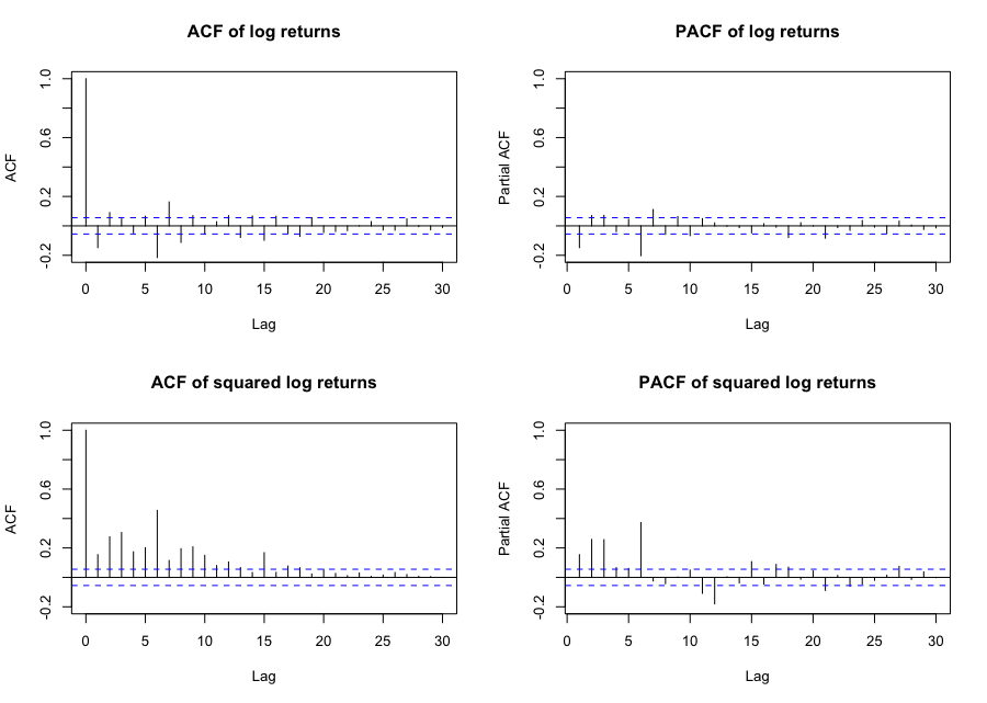
See A3 for the code to generate this figure.

It is not so easy to determine the orders of a GARCH model by looking at the results of ACF and PACF in Figure $3$, since they show significant (partial) correlations at multiple lags without clear decay. In such cases, it is standard to start with a simple model, GARCH $(1, 1)$, and examine the dependence structure of the squared standardized residuals from the fitted GARCH model using ACF and PACF plots. The standardized residual from GARCH model is the estimated White Noise term, $\hat{W_{t}}$ and is defined as

$\hat{W_{t}} = \dfrac{E_{t}}{\hat{\sigma}_{t}} \tag{13}$

When the square of these show a significant dependence structure, it indicates that the model is not capturing all the dynamics of the time series. In this case, we can consider increasing the order of the GARCH model and refitting it to the data until the dependence structure becomes not significant.

The conditional variance, $\sigma_{t}^{2}$, from GARCH $(1, 1)$ model is defined as

$\sigma_{t}^{2} = \alpha_0 + \alpha_1 E_{t-1}^{2} + \beta_1 \sigma_{t-1}^2 \tag{14}$

We can estimate this model using the garchFit() function in the R library fGarch.

library(fGarch)
heavy_fit <- garchFit(~garch(1, 1), MCD_lreturn, cond.dist="std")

The parameter cond.dist=std specifies that the White Noise innovations, $W_{t}$, in the GARCH model are assumed to follow a standardized $t$ -distribution. The estimated results of the GARCH $(1, 1)$ model for the log returns of McDonald’s stock are as follows.

All of the parameter estimates in Equation 15, for $\mu$, $\alpha_0$, $\alpha_1$, $\beta_1$, and $v$ in Equations 8, 10, and 14, are statistically significant at a 5% significance level. I have also tested higher orders, but those are not statistically significant at any meaningful statistical level.

Now, we calculate the squared standardized residuals of the fitted model according to Equation $13$ and plot ACF and PACF of these.

st_resid <- heavy_fit@residuals / heavy_fit@sigma.t

par(mfcol=c(1,2))
acf(st_resid^2, ylim=c(-0.2,1), main="")
pacf(st_resid^2, ylim=c(-0.2,1), main="")

Figure 4. ACF (left) and PACF (right) of the squared standardized residuals from the fitted GARCH $(1, 1)$ model. There is no significant serial dependence anymore.

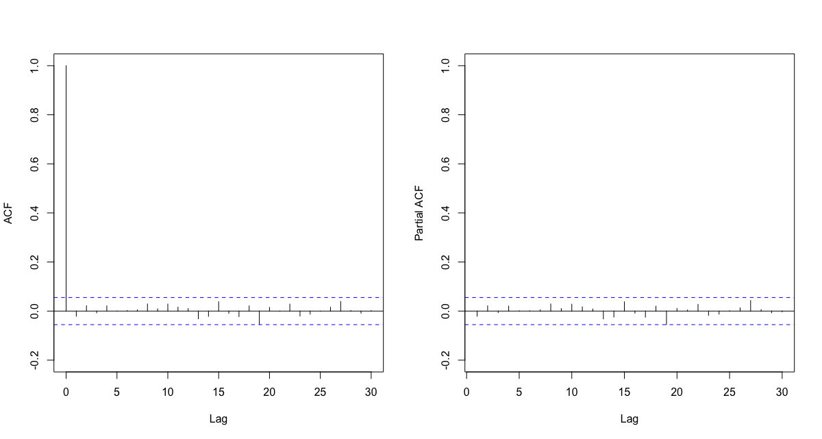
Since the squared standardized residuals, or the estimated White Noise innovations, $\hat{W}_{t}$, do not show any significant autocorrelation, GARCH $(1, 1)$ is sufficient to capture all the dynamic volatility in the log returns of McDonald’s stock.

We can also check if the $t$-distribution is a right choice to model the tail behavior of our log returns using qqplots.

Figure 5. A comparison between the QQplot of log returns with $t$-distribution (left) and the QQplot of log returns with Gaussian distribution (right) shows that the $t$-distribution is better at capturing the heavy-tailed behavior of the log returns of McDonald's stock.

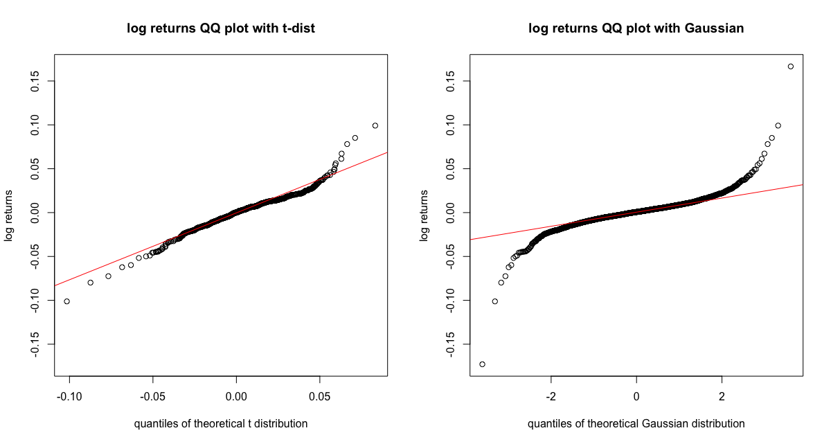
See A4 for the code to generate this figure.

Daily VaR with GARCH

Now, let’s calculate daily VaR of McDonald’s stock. With the estimated GARCH $(1, 1)$ model in Equation $15$, the predicted conditional standardized deviation, $\hat{\sigma}_{t}$, right after 2023-01-01 is calculated in R as

> predict(heavyt_fit, n.ahead=1)$standardDeviation
[1] 0.01581185

Let’s add the estimated conditional standard deviation to the estimated results from GARCH $(1, 1)$ in Equation $15$.

We can think of our estimated log return at time $t$, $\hat{X}_{t}$, as a random variable from a non-standardized $t$-distribution with mean of $0.0006$ and variance of $0.016^{2}\times \dfrac{4.7}{4.7-2}$, which could be written as $t_{4.7} \left(0.0006, 0.016^{2}\cdot \dfrac{4.7}{4.7-2} \right)$. It is because $\hat{W}_{t}$ follows a standardized $t$-distribution with $4.7$ degrees of freedom, $t_{4.7} \left(0, \dfrac{4.7}{4.7-2}\right)$.

But usually, when using $t$-distribution for GARCH modeling, we convert the estimated conditional standard deviation, $\hat{\sigma}_{t}$ by multiplying it by the inverse of the estimated standard deviation of the standardized $t$-distribution, $\sqrt{\dfrac{\hat{v}-2}{\hat{v}}}$, which in our case is $\sqrt{\dfrac{4.7-2}{4.7}}$.

This is to cancel the variance of the standardized $t$-distribution, $\dfrac{v}{v-2}$. There are two reasons for doing so. $1)$ We want our modeled time-series, $\hat{X}_{t}$ to have the same conditional variance as the one estimated from the GARCH model, which in our case is $0.016^{2}$. $2)$ We want to avoid the problem of not being able to calculate the variance of the standardized t distribution when the degrees of freedom are less than or equal to 2. It is because the standardized $t$-distribution has its finite variance, $\dfrac{v}{v-2}$, only when $v>2$.

We can calculate the VaR with a $95\%$ confidence level from the estimated model in Equation $17$ using R as follows.

df <- coef(heavy_fit)["shape"]
adjusted_sd <- sqrt((df-2)/df) * (predict(heavyt_fit, n.ahead=1)["standardDeviation"])
mu <- coef(heavy_fit)["mu"]

mu + adjusted_sd * qt(0.05, df)
1       -0.02384826

The one period (daily) Value at Risk of the log returns of McDonald’s stock over the past five years with a confidence level of $95\%$ is about $-2.385\%$. In other words, we are $95\%$ confident in the fact that our daily maximum expected loss right after 2023-01-01 is less than about $2.385\%$.

Appendix

A1: Prices, simple returns and log returns plots

I imported the closing price data of McDonal’s stock for the past five years from Yahoo Finance through getSymbols function in quantmod library.

# load Mcdonald's stock data
library(tidyquant)

options("getSymbols.warning4.0"=FALSE)
options("getSymbols.yahoo.warning"=FALSE)

getSymbols("MCD", from = '2018-01-01',
           to = "2023-01-01",warnings = FALSE,
           auto.assign = TRUE)


# price, return, log return into one xts object
MCD <- MCD[, "MCD.Close"]
MCD_sreturn <- diff(MCD)/stats::lag(MCD)  ## dplyr::lag(MCD) generates error
MCD_lreturn <- diff(log(MCD))
MCD_lreturn <- na.omit(MCD_lreturn)

MCD_perform <- merge(MCD, MCD_sreturn, MCD_lreturn)
colnames(MCD_perform) <- c("Price", "Simple_return", "Log_return")


# plot the three
library(ggplot2)

autoplot(MCD_perform) +
  xlab("Year") +
  scale_x_date(date_breaks = "1 year") +
  facet_grid(Series ~ ., scales="free_y",
             switch="y") +
  theme(strip.background = element_blank(),
        panel.background = element_blank(),
        panel.grid.major =  element_line(colour="#E7E7E7"),
        panel.grid.minor = element_line(colour="#E7E7E7"),
        axis.line = element_line(colour = "black"),
        strip.placement = "outside",
        strip.text = element_text(size = 14),
        axis.title.x = element_text(size = 14),
        axis.text = element_text(size=14)) +
  geom_line(color="#1F77B4", size=0.5)

A2: Empirical VaR plot

# plot 1-period empirical VaR with confidence of 95%
VaR <- quantile(MCD_lreturn, 0.05)

hist(returns, breaks = 50, col = "#1F77B4", main = "", xlab = "Daily Log Return",
     ylab = "Frequency", ylim=c(0, 650))
abline(v = VaR, col = "#D62728", lwd = 2, lty = 2)
legend("topright", legend = paste0("VaR (95% confidence): ", round(VaR * 100, 2),
                                   "%"), col = "#D62728", lty = 2, cex = 0.8)

A3: ACF and PACF plot

MCD_lreturn_sq <- MCD_lreturn^2
par(mfcol=c(2,2))
acf(MCD_lreturn, ylim=c(-0.2,1), main="ACF of log returns")
acf(MCD_lreturn_sq, ylim=c(-0.2,1), main="ACF of squared log returns")
pacf(MCD_lreturn, ylim=c(-0.2,1), main="PACF of log returns")
pacf(MCD_lreturn_sq, ylim=c(-0.2,1), main="PACF of squared log returns")

A4: QQplots with two distributions

par(mfcol=c(1, 2))
## qqplot with t-dist
df <- coef(heavy_fit)["shape"]
theo_t_quantiles <- sort(coef(heavy_fit)["mu"]+ 
                           heavy_fit@sigma.t * qt(seq(0, 1, length=length(MCD_lreturn)), df=df))

plot(theo_t_quantiles, sort(coredata(MCD_lreturn)), 
     main="log returns QQ plot with t-dist", 
     xlab="quantiles of theoretical t distribution", 
     ylab="log returns")

## qqline with t-dist
a <- quantile(MCD_lreturn, probs=c(0.25, 0.75))
b <- coef(heavy_fit)["mu"]  + 
  quantile(heavy_fit@sigma.t * 
             qt(seq(0, 1, length=length(MCD_lreturn)), df=df), probs=c(0.25, 0.75))

slope <- diff(a)/diff(b)
intercept <- a[1] - slope*b[1]

abline(intercept, slope, col="red")

## qqplot and qqline with Gaussian
qqnorm(MCD_lreturn, 
       main = "log returns QQ plot with Gaussian", 
       xlab="quantiles of theoretical Gaussian distribution", 
       ylab="log returns")

qqline(MCD_lreturn, col="red")